If you have not studied some basics of "Python" for data science, please take a short tour to "Learnin Python in 90 minutes", which gives you a concise tutorial of "Python", "NumPy", and "pyplot".

We here use "Anaconda", a software package of Python, for further tutorials on data science. Please follow the installation instructions at Official Page of Anaconda. Choose your platform (Windows, macOS, Linux) and download the installer for the latest version of Python 3 (3.6 or later). For macOS, "Graphical Installer" would be easy to handle. For Windows, "64-bit" would be appropriate in most cases. For Linux, choose "64-bit" for X86.

After installation, open a "Terminal" window, make a directory for our project (say, "jupyter") and move into that directory. This can be done by the following procedure. (Note: The text in red is what you need to type in.)

yourPC> mkdir jupyter
yourPC> cd jupyter

Now, let us start "jupyter" by typing "jupyter notebook" on the terminal.

yourPC> jupyter notebook

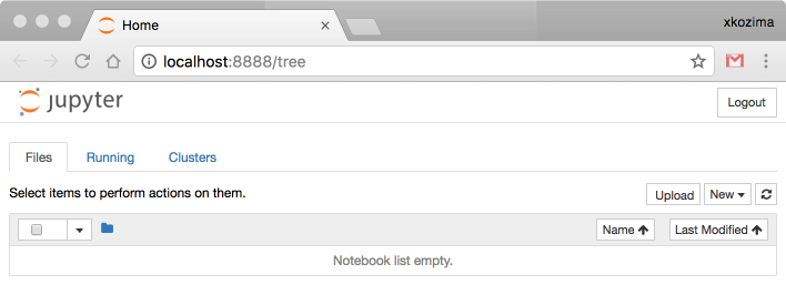
Hopefully, your default browser (preferably Chrome, Firefox, or Safari; but not IE or Edge) opens automatically some starting page of "jupyter". It should look like the following.

Jupyter notebook is an interactive development environment especially suitable for data analysis using Python. Your code runs on the Python interpreter on your PC, and your web browser works as an interactive interface for coding and visualizing. You could also use Jupyter notebook as a frontend for programming in other languages, like JavaScript or R.

So far, your notebook may be empty. Let us make a new one, by clicking "new" and choose "Python3" from the menu. You will have a new tab, in which you can run any Python script interactively.

Try copy the following Python code and paste it on your notebook (to the right side of "In [ ]:".

import numpy as np
import matplotlib.pyplot as plt

x = np.arange(-4.0, 4.0, 0.02)
plt.plot(x, np.sin(x), label="source")
plt.plot(x, np.sin(10*x), label="carrier")
y = np.sin(x) * np.sin(x * 10.0)
plt.plot(x, y, label="modulated", linewidth="2")

plt.legend()
plt.title("AM (amplitude modulation)")
plt.show()

Then, type "Control-enter" to run the code. The results, even the graphs, are just shown below the code. Try it out!

If you want the graph plotted in higher resolution, place "plt.savefig('filename.png', dpi=600)", for example, right after "plt.show()". You will get a png file in higher resolution (600 dots per inch) in the directory "~/jupyter".

If you want to leave the code and result above and proceed to make another interaction, just click "+" icon on the tool bar. You will have a new input area, called a "cell", where you can type in a new code to run. This example generates a histogram of 100 random numbers in normal (Gaussian) distribution (μ=0, SD=1).

Note that Python takes the new code (In [2], here) as in the succeeding environment of the past interactions. So, you do not need to re-import "numpy" or "pyplot" in here. All variables and functions are succeeded from the preceeding interaction. Try out the following code in a new cell. It enlarges the number of the random numbers. It succeeds the varible "bins" from the previous interaction. Try changing the number of samples to (1000, 10000, 100000, etc.) and see how the histogram is shaped into.

Because it is a "notebook", you can add texts to explain what you are doing, or recording what you have found. To do that, just add a "Cell" by clicking "+", then change its type from "Code" to "Markdown", and type in what ever you want to show. If you want to make the text bigger for headlines, try "# My Huge Header", "## My Large Header", "### My Header", and so on. You can use HTML tags in the markdown.

You can save the notebook (codes and results), by just clicking the "floppy-disk" icon or just typing "Command-S" or "Control-S" on the browser. So far, your notebook is temporarilly named as "Untitled". You can rename it by opening "File" menu and choose "rename". Now you can close the browser tab or quit the browser. The actual filename looks like "filename.ipynb", where "ipynb" stands for "IPython notebook". "IPython" is the former name of "jupyter".

When you want to resume your interaction with the saved notebook, start your browser and open URL "localhost:8888/tree". You will see the contents of the "jupyter" directory. Clicking the filename you have just saved, you will get the entire notebook opened. (It is recommended to bookmark "localhost:8888/tree" for convenience.)

Please download my notebook "perceptron.ipynb" and put it in the "jupyter" directory. Start "jupyter" by typing "jupyter notebook" in a terminal window. You will see the notebook on your browser. It's ready to interact with the notebook.